Introduction
 |
Radiosity is a finite element method that computes a
view independent GI solution as a finite mesh.
The environment is divided up into patches that are uniform and
perfectly diffuse and energy is transferred amongst these patches until
equalized. This tight coupling of
the lighting information to the geometry is costly to calculate and meshing
artifacts can occur if not carefully constructed.
Radiosity also doesn’t handle arbitrary reflection models.
Path tracing is a probabilistic view dependent point sampling technique that extends raytracing to approximate all light paths such as those that contribute to indirect illumination and caustics. The scene is rendered by tracing a set of ray paths from the eye back to the lights, where each path does not branch. Path tracing is a random process where each path is a simple random walk and thus a Markov chain. Path tracing can be very computationally expensive as a large number of samples are needed to converge or variance will show up as noise in the final image. |
Fortunately,
Photon Mapping is a two pass global illumination
algorithm developed by Henrik Jensen as an efficient alternative to pure
In this write-up I plan to give an over-view of the two passes of Photon Mapping. I will not touch upon participating media and the various optimizations relating to photon mapping and uses in other algorithms.
First Pass - Photon Tracing
Photon Emission
A photon’s life begins at the light source. For each light source in the scene we create a set of photons and divide the overall power of the light source amongst them. Brighter lights emit more photons then dimmer lights. Finding the number of photons to create at each light depends largely on whether decent radiance estimates can be made during the rendering pass. For good radiance estimates the local density of the photons at surfaces need to provide a good statistic of the illumination.
|
|
| Figure recreated from [1] |
Jensen states that any type of light source can be used and describes several emission models. For point light sources we want to emit photons uniformly in all directions. For area light sources we pick a random position on the surface and then pick a random direction in the hemisphere above this position.
Photon Scattering
Emitted photons from light sources are scattered through a scene and are eventually absorbed or lost. When a photon hits a surface we can decide how much of its energy is absorbed, reflected and refracted based on the surface’s material properties.
It is important to note that the power of the reflected photon is not modified. Correctness of the overall result will converge with more samples. The probability is given by the reflectivity of a surface. If the reflectivity for a surface is 0.5 then 50% of the photons will be reflected at full power while the other 50% will be absorbed. To show why Russian Roulette reduces computational and storage costs let’s consider shooting 1000 photons at a surface with reflectivity of 0.5. We could reflect 1000 photons at half power or we can reflect 500 at full power using Russian Roulette.
Considering only diffuse and specular reflection and absorption we have the following domain
Photon Storing
For a given scene we may shoot millions of photons from the light sources. It is desirable that our photon map is compact to reduce the storage costs. We also want it to support fast three dimensional spatial searches as we will need to query the photon map millions of times during the rendering phase.
The data structure that Jensen recommends using for the photon map is a kd-tree. It is one of the few data structures that is ideal for handling non-uniform distributions of photons. The worst-case complexity of locating photons in a kd-tree is O(n) where as if it is balanced it is O(log n). After all photons are stored in the map we want to make sure it is balanced.
For each photon we store its position, power, and incident direction. Jensen proposes the following structure.
struct
photon {
float x, y, z;
// position ( 3 x 32 bit floats )
char p[4];
// power(rgb) packed as 4 chars
char phi, theta;
// compressed incident direction
short flag;
// flag used for kd-tree
}
Jensen prescribes Ward’s shared-exponent RGB format for packing the power into 4 bytes. The phi and theta are spherical coordinates that mapped to 65536 possible directions. The position can possibly be compressed further into a 24bit fixed point format.
However, for most serious implementations the structure will be as compressed as possible to allow for extremely large and complex scenes. For naďve renderers the structure can remain largely uncompressed for ease of use.
Second Pass - Rendering
Approximating the Rendering Equation
In order to get a good radiance estimate we need a sufficient number of photons in our density estimate. Of course this can directly relate to the number of photons that are emitted from the light sources. The more photons that are used the more accurate is our estimate. We also need to be careful how we collect photons.
The main idea behind gathering photons is that we are hoping to get an idea of what the illumination at x is by examining the nearest N photons. If we include photons from other surfaces, with drastically different surface normals, or from volumes in our estimate then we can degrade the accuracy of our estimate.
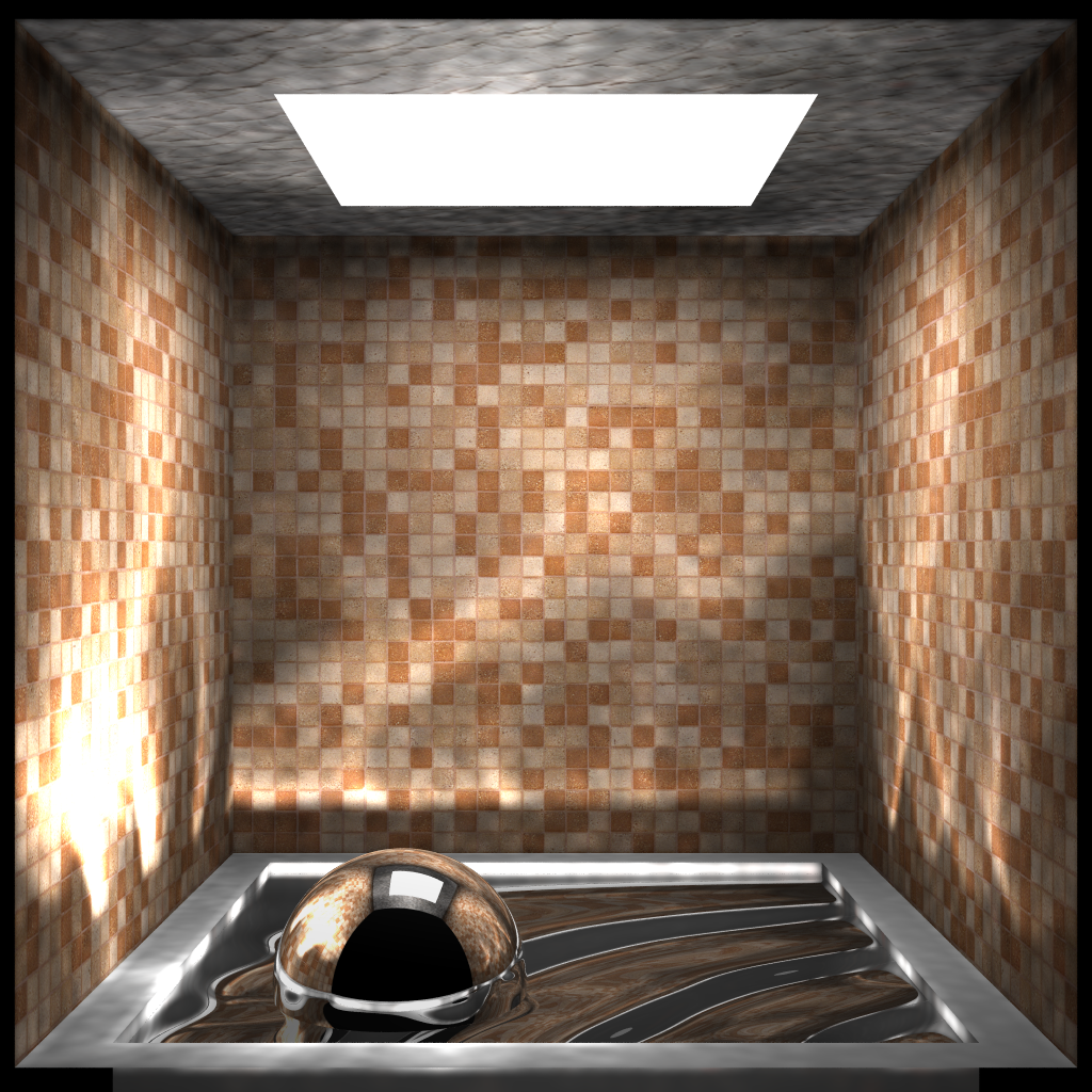
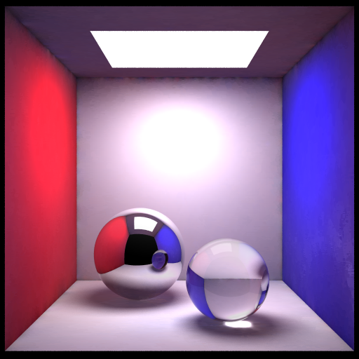
Caustics
click on images to enlarge
|
|
|
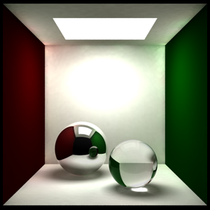
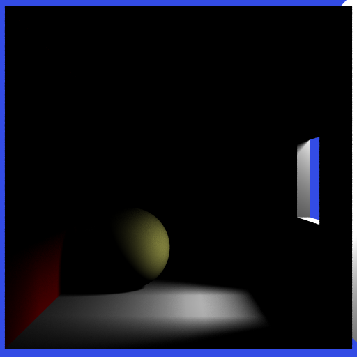
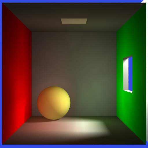
Indirect Illumination
However, even without a final gather step it is possible to achieve images such as the one below. The image on the left shows the contribution from direct lighting only and the image on the right was rendered using photon mapping. The image on the right does not use a final gather step. Only 26,000 photons actually made it into the window and 500 were used in the radiance estimate. Notice the color bleeding on the yellow ball and on the floor.
click on images to enlarge
|
|
|
click on images to enlarge
|
|
|

Flexibility
Due to the fact that information from the photon map describes the incoming flux and that this information is decoupled from the geometry we have the flexibility to solve different parts of the rendering equation by using multiple photon maps. This is also another reason why photon mapping can easily be incorporated into existing renderers.
For example, we may have an existing path tracer where we would like to use photon mapping to handle caustics. Path tracing does a great job at computing the direct and indirect lighting while photon mapping handles caustics which removes the high frequency noise typically seen in path traced images. In addition, we can use information from the photon map to help us importance sample the hemisphere.
Another great feature of the photon maps is that it provides information that can be used as heuristics for other parts of the rendering equation. For example, with a little extra work, information from the photon map can provide information as to whether shadow rays are needed at a location. This alone can reduce the rendering times significantly. In path tracers the photon map can also be used for importance sampling.
References
| [1] | Jensen, Henrik W., Realistic Image Synthesis Using Photon Mapping, A K Peters, Ltd., Massachusetts, 2001 |
| [2] | Shirley, Peter Realistic Raytracing A K Peters, Ltd. Massachusetts, 2000. |
| [3] | James T. Kajiya. The Rendering Equation. Computer Graphics, 20(4):143-150, August 1986. ACM Siggraph ’86 Conference Proceedings. |
| [4] |
Shirley, Peter Fundamentals of Computer Graphics, A K Peters, Ltd, Massachusetts, 2002 |
| [5] | Glassner, Andrew Principles of Digital Image Synthesis Morgan Kaufmann Publishers, Inc., San Fransico, 1995 |
| [6] | Ward et al, A Ray Tracing Solution for Diffuse Interreflection.Computer Graphics, 22(4): 85-92 August 1988. ACM Siggraph '88 Conference Proceedings. |