John Pawasauskas
CS563 - Advanced Topics in Computer
Graphics
February 18, 1997
Ray casting is a method used to render high-quality images of solid objects.
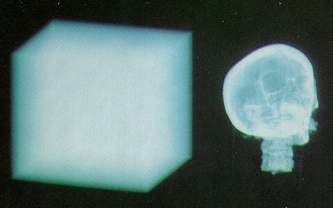
The term volume rendering is used to describe techniques which allow the visualization of three-dimensional data. Volume rendering is a technique for visualizing sampled functions of three spatial dimensions by computing 2-D projections of a colored semitransparent volume.
Currently, the major application area of volume rendering is medical imaging, where volume data is available from X-ray Computer Tomagraphy (CT) scanners and Positron Emission Tomagraphy (PET) scanners. CT scanners produce three-dimensional stacks of parallel plane images, each of which consist of an array of X-ray absorption coefficients. Typically X-ray CT images will have a resolution of 512 * 512 * 12 bits and there will be up to 50 slides in a stack. The slides are 1-5 mm thick, and are spaced 1-5 mm apart.
In the two-dimensional domain, these slides can be viewed one at a time. The advantage of CT images over conventional X-ray images is that they only contain information from that one plane. A conventional X-ray image, on the other hand, contains information from all the planes, and the result is an accumulation of shadows that are a function of the density of the tissue, bone, organs, etc., anything that absorbs the X-rays.
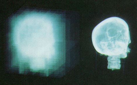
The availablilty of the stacks of parallel data produced by CT scanners prompted the development of techniques for viewing the data as a three-dimensional field rather than as individual planes. This gave the immediate advantage that the information could be viewed from any view point.
There are a number of different methods used:
There are some problems with the first two of these methods. In the first method, choices are made for the entire voxel. This can produce a "blocky" image. It also has a lack of dynamic range in the computed surface normals, which produces images wit relatively poor shading.
The marching cubes approach solves this problem, but causes some others. Its biggest disadvantage is that it requires that a binary decision be made on the position of the intermediate surface that is extracted and rendered. Also, extracting an intermediate structure can cause false positive (artefacts that do not exist) and false negatives (discarding small or poorly defined features).
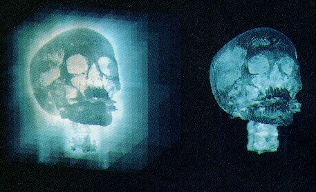
The basic goal of ray casting is to allow the best use of the three-dimensional data and not attempt to impose any geometric structure on it. It solves one of the most important limitations of surface extraction techniques, namely the way in which they display a projection of a thin shell in the acquisition space. Surface extraction techniques fail to take into account that, particularly in medical imaging, data may originate from fluid and other materials which may be partially transparent and should be modeled as such. Ray casting doesn't suffer from this limitation.
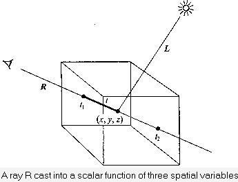
Currently, most volume rendering that uses ray casting is based on the Blinn/Kajiya model. In this model we have a volume which has a density D(x,y,z), penetrated by a ray R.
At each point along the ray there is an illumination I(x,y,z) reaching the point (x,y,z) from the light source(s). The intensity scattered along the ray to the eye depends on this value, a reflection function or phase function P, and the local density D(x,y,z). The dependence on density expresses the fact that a few bright particles will scatter less light in the eye direction than a number of dimmer particles. The density function is parameterized along the ray as:
D(x(t), y(t), z(t)) = D(t)
and the illumination from the source as:
I(x(t), y(t), z(t)) =
I(t)
and the illumination scattered along R from a
point distance t along the ray is:
I(t)D(t)P(cos
Ø)
where Ø is the angle between R and
L, the light vector, from the point of interest.
Determining I(t) is not trivial - it involves computing how the radiation from the light sources is attenuated and/or shadowed due to its passing through the volume to the point of interest. This calculation is the same as the computation of how the light scattered at point (x,y,z) is affected in its journey along R to the eye. In most algorithms, however, this calculation is ignored and I(x,y,z) is set to be uniform throughout the volume. For most practical applications we're interested in visualization, and including the line integral from a point (x,y,z) to the light source may actually be undesirable. In medical imaging, for example, it would be impossible to see into areas surrounded by bone if the bone were considered dense enough to shadow light. On the other hand, in applications where internal shadows are desired, this integral has to be computed.
The attenuation due to the density function along a ray can be calculated
as:
where  is a constant that
converts density to attenuation.
is a constant that
converts density to attenuation.
and the intensity of the light arriving at the eye along direction R due to all the elements along the ray is given by:
When it pertains to volume visualization, ray casting is often referred to as ray tracing. Strictly speaking this is inaccurate, since the method of ray tracing with which most people are familiar is more complex than ray casting. However, the basic ideas of ray casting are identical to those of ray tracing, and the results are very similar.
Algorithms which implement the general ray casting technique described above involve a simplification of the integral which computes the intensity of the light arriving at the eye. The method by which this is done is called "additive reprojection." It essentially projects voxels along a certain viewing direction. Intensities of voxels along parallel viewing rays are projected to provide an intensity in the viewing plane. Voxels of a specified depth can be assigned a maximum opacity, so that the depth that the volume is visualized to can be controlled. This provides several useful features:
Additive reprojection uses a lighting model which is a combination of reflected and transmitted light from the voxel. All of the approaches are a subset of the model in the following figure.
In the above figure, the outgoing light is made up of:
Several different algorithms for ray casting exist. This presentation will describe the implementation presented by Marc Levoy in many of his papers, which is used in several commercial applications.
For every pixel in the output image, a ray is shot into the data volume. At a predetermined number of evenly spaced locations along the ray the color and opacity values are obtained by interpolation. The interpolated colors and opacities are then merged with each other and with the background by compositing in either front-to-back or back-to-front order to yield the color of the pixel. (The order of compositing makes no difference in the final output image.)
Levoy describes his technique as consisting of two pipelines - a visualization pipeline and a classification pipeline. The output produced by these two pipelines is then combines using columetric compositing to produce the final image.
In the visualization pipeline the volume data is shaded. Every voxel in the data is given a shade using a local gradient approximation to obtain a "voxel normal." This normal is then used as input into a standard Phong shading model to obtain an intensity. The output from this pipeline is a three color component intensity for every voxel in the data set.
Note that in completely homogeneous regions the gradient is zero. The shade returned from such reasons is unreliable. To solve this problem, Levoy based the opacity of each voxel on the gradient. The gradient is multiplied by the opacity. Homogeneous regions have an opacity of zero, and thus do not affect the final image.
The classification pipeline associates an opacity with each voxel. The color parameters which are used in the shading model are also used in this pipeline. The classification of opacity is context dependent, and the application of Levoy's technique is in X-ray CT images (where each voxel represents an X-ray absorption coefficient).
We now have two values associates with each voxel:
 (X) - an
opacity derived from tissue type of known CT values
(X) - an
opacity derived from tissue type of known CT valuesThe next stage, volumetric compositing, produces a two-dimensional
projection of these values in the view plane. Rays are cast from the eye to the
voxel, and the values of C(X) and
(X) are "combined"
into single values to provide a final pixel intensity.
For a single voxel along a ray, the standard transparency formula is:

where:
Cout
is the outgoing intensity/color for voxel X along the ray
Cinis
the incoming intensity for the voxel
It is possible to interpolate from the vertex values of the voxel which the ray passes through, but it's better to consider neighboring voxels (8 or 26) and trilinearly interpolate. This yields values that lie exactly along the ray.
Ultimately, this yields the following pseudocode:
There are a number of visualization packages which provide ray casting capabilities. These include:
There are a number of other packages which support ray casting as well, including many non-commercial visualization systems. Interestingly, SGI's IRIS Explorer doesn't provide a ray casting feature, instead supplying other methods for volume visualization.
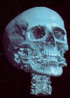
There are many example images to be found which illustrate the capabilities of ray casting. These images were produced using IBM's Data Explorer.

Ray casting is an extremely computation intensive process, much like ray tracing is. And like ray tracing, there are a number of optimization techniques which can be used to increase the speed with which an image can be rendered.
This is the first optimization technique for ray casting algorithms. If we
have a dataset measuring N voxels on a side, and where
N = 2M+1
for some integer M, we can represent this enumeration by a pyramid of M+1 binary
volumes. Volumes in this pyramid can be indexed by a level number m
where m= 0,...M, and the volume at level m is denoted by Vm.
Volume V0 measures N-1 cells on a side, volume V1measures
(N-1)/2 cells, and so on, up to volume Vm which is a single
cell.
Cells are indexed by a level number m and a vector i=(i,j,k) where i,j,k = 1,...,N-1 and the value contained in cell i on level m is denoted Vm(i). The size of the cells on level M is defined to be 2m times the spacing between voxels. Voxels are treated as points, and cells fill the space between voxels. Thus, each volume is one cell larger in each direction than the underlying dataset. Voxel (1,1,1) is placed at the front-lower-right corner of cell (1,1,1). Thus, cell (1,1,1) on level zero encloses the space between voxels (1,1,1) and (2,2,2).
To construct the pyramid, we do the following: Cell i in the base volume V0 contains a zero if all eight voxels lying at its vertices have opacity equal to zero. Cell i in any volume Vm, m>0, contains a zero if all eight cells on level m-1 that form its octants contain zeros.
To state this differently, let {1,2,...,k}n be the set of all
n-vectors with entries {1,2,...,k}. Since we're concerned with
three-dimensional data, we only care about the condition where n=3. This gives
us {1,2,...,k}3, which is the set of all vectors in 3-space with
integer entries between 0 and k. Then, we can define
and
where m=1,...,M.
We have to reformulate the ray casting, resampling, and compositing steps of the rendering algorithm to use this pyramidal data structure. For each point, we first compute the point where the ray enters the single cell at the top level. We then traverse the pyramid in the following manner: When we enter a cell, we test its value. It if contains a zero, we advance along the ray to the next cell on the same level. If the parent of the new cell differs from the parent of the old cell, we move up to the parent of the new cell. We do this because if the parent of the new cell is unoccupied we can advance the ray farther on our next iteration than if we had remained on a lower level. This ability to quickly advance across empty regions of space is where the algorithm saves its time. On the other hand, if the cell being tested contains a one, we move down one level, entering whichever cell encloses our current location. If we are already at the lowest level, we know that one or more of the eight voxels at the vertices of the cell have opacity greater than zero. We then draw samples at evenly spaced locations along that part of the ray falling within the cell, resample the data at these sample locations, and composite the resulting color and opacity into the color and opacity of the ray.
The following image shows in two dimensions how a typical ray may traverse a
heirarchical enumeration.
The goal of adaptive terminationis to quickly identify the last sample along
a ray that significantly changes the color of the ray. We define a significant
color change as one in which Cout - Cin > Epsilon for
some small Epsilon > 0. Thus, Once
first exceeds 1-Epsilon,
the color will not change significantly. This is the termination criteria.
Higher values of Epsilon reduce rendering time, while lower values of Epsilon reduce image artifacts producing a higher quality image.
By combining the two optimization methods, we can further increase the
performance gain. The two methods are combined in the following algirithm:
In the above algorithm, the Index function accepts a level number and the object-space coordinates of a point, and returns the index of the cell that contains it. The Parent function accepts a level number and cell index, and returns the index of the parent cell. The Next function accepts a level number and a point on a ray, and computes the coordinates of the point where the ray enters the next cell on the same level. The RenderCell function composites the contribution made to a ray by the specified interval of volume data. The algorithm terminates when the ray exits the data as detected by the InBounds procedure.
In this section, there are several sample images, as well as some tables
which convey some data about the images. There is also a cost comparison of
normal "brute force" ray casting, ray casting using heirarchical
enumeration, and ray casting using heirarchical enumeration and adaptive
termination.
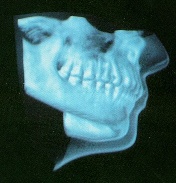 Jaw with skin
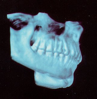 Jaw without skin
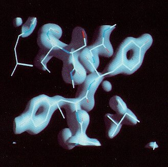 Ribonuclease
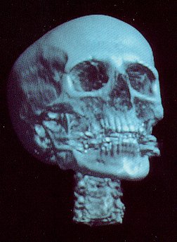 Head
Head
 Brute force
 Heirarchical enumeration
 Heirarchical
enumeration and adaptive termination
Heirarchical
enumeration and adaptive termination
Copyright © 1997 by John Pawasauskas