Spectral BRDF

CS 563 Advanced Topics in Computer Graphics: Spectral BRDF
Cliff Lindsay - Spring, 2003 WPI

Spectral Rendering is a recent trend in Computer Graphics that arose from efforts to render scenes and images in a more physically based fashion. There are phenomenons that exist in nature that cannot be rendered using the conventional RGB representation of color. Therefore, if we try and recreate physically accurate scenes, we need to render these images with their spectra instead of an approximate RGB values. This paper will discuss the following relevant topics: color theory, tone mapping (i.e., tone reproduction), mapping spectra to color and vice versa, and spectral BRDFs.

When rendering images using Spectra instead of RGB values, we are still plagued with the problem of converting spectra to RGB values when displaying out images to a conventional display device (CRT, LCD, etc.). Color theory helps inform us of our options for converting Spectra to color, covers well-known standards, and why these standards are a good physical fit for various situations. Tone mapping or Tone Reproduction helps take physically known or measured spectral values and maps their attributes to display devices that evoke similar responses expected in a natural environment. These techniques usually arise from the limitations of software, hardware, and even human eyes can only display low range values for spectra.

At times, situations arise when there is a need to proceed in reverse order and reproduce unknown spectra from known RGB values. There are a couple of techniques for doing this that are briefly discussed in section 4. The final topic will focus on examples implementing the previously mentioned techniques for rendering natural phenomenon such as florescence, dispersion, and interference of light.

Color theory stems from the idea that light has various wave-like properties. These wave-like properties allow us to categorize light by measurements made on a gradient scale called the visual spectrum scale. Other scales exist that stem from a relationship with the Human Visual System and color spectra. These scales are often referred to as Tristimulus scales. For example, in 1931, a French organization called Commission Internaionale de l'Eclairage developed a standard scale called CIE XYZ that is based on the Tristimulus system. The Tristimulus system relies on weighted values of completely Red, Green, and Blue spectral curves to represent all colors.

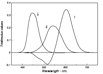
Figure 1. Graph of the color matching functions for RGB primaries[hill01].

The color we see in everyday objects results from a Dominant wavelength in that object's color spectrum. The Dominant wavelength is the part of the object's spectral curve that contributes the most to that wavelength. In other words, the more a color exists in an object, the more that object will have that color. CIE XYZ takes these properties and produces a mathematical representation of the Spectra in the form of an Integral for each stimulus wavelength (RGB).

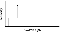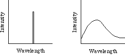
Figure 2. Examples of different spectra displaying dominat wavelength[hill01].

Although each of us can perceive colors slightly differently, the CIE has defined a standard observer. A set of standard conditions for performing color measuring experiments has also been proposed by CIE. A number of color matching experiments have been performed under these standardized conditions. Color matching experiments consists of choosing three particular light sources, that emit light on the white screen, where three projections overlap and form an additive mixture.On the other side of the screen a target color is projected, and an observer tries to match the target light by altering the intensities of the three light sources. The weights of light sources are in the range [-1,1]. Negative weights are allowed, as it is not possible to match all colors using only positive weights. A negative weight does not mean subtracting color from the additive mixture, but rather adding this color to the target color. After many experiments using light sources of the wavelengths red=700 nm, green=546.1 nm and blue is 435.8 nm color matching curves as shown in figure 3 were proposed by CIE [WySt82].

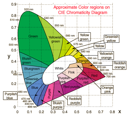
Figure 3. CIE XYZ Chart

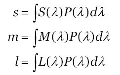
Figure 4. Color Matching Functions.

3. Tone mapping (Tone Reproduction)

Tone Mapping is a technique for scaling luminance values of a real world scene into a range that is displayable on an output device (monitor, LCD, printer, etc.). Whereas the human visual system ranges from 100 to 1 Candelas, the luminance range for a real outdoor scene is 100 million to one. The goal of Tone mapping is to mimic the perceptual qualities of a real world scene. Tone mapping can be segregated into three types of techniques, Spatially Uniform (global), Spatially Varying (local), and Time Variant. Spatially Uniform Tone Mapping attempts to map the appropriate Luminance levels of a whole scene, where as Spatially Varying Tone Mapping will to map Luminance levels of a local area, and Time Variant Tone Mapping changes over time.

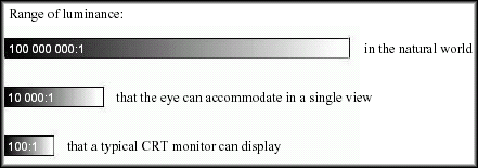
Figure 5. A comparative view of dynamic range[devlin02].

Tone mapping operators try to reproduce the image in such a a way that the resulting mental image is as close as possible (identical) to the mental image of the real environment. They work on LUMINANCES i.e. they are greyscale only. Most extensions to colour spaces are heuristics only.

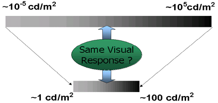
Figure 6. Due to the adaptation mechanisms of the HVS we can reproduce subjective brightness and contrast even if we cannot reproduce the bright luminance scale[mcnamara01].

Spatially Uniform Tone Mapping techniques have been developed to incorporate a wide variety of scale to measure, compare and contrast luminance values throughout the scene. One technique for luminance mapping is called a linear technique, where the highest luminance value in the scene is mapped directly to the highest luminance value on the display device. Other techniques, such as low curvature, log-log scales, and log-linear scales, use more sophisticated algorithms for mapping luminance values. In a research paper by Kate Devlin entitled "A review of tone reproduction techniques", 2002, there is a table that describes the various scales that have been developed for Spatially Uniform Tone mapping (as well as Spatially Varying Tone Mapping, and Time Variant Tone Mapping).

The image on the left of Figure 7 presents a simple min-max operator that scales the dynamic range of the radiance data to the dynamic range of the output format. The image on the right uses Ward's tone mapping operator.

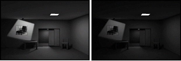
Figure 7. Tone-reproduction operator performs a linear scaling to preserve the contrast[ward94].

Spatially Varying Tone Mapping tries to match the luminance values from a small area in a scene to a scale that is within the range of the output device. This technique works well for scenes that normally have low luminance variation except in a small region of the scene. Spatially Varying Tone Mapping techniques incorporate various types of scales similar to that of Spatially Uniform Tone Mapping such as simple linear, zone systems, and log type scales.

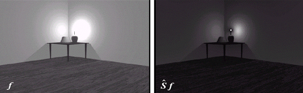
Figure 8. Original image vs. Image with blurring and and inversion scaling[chui93].

Time Variant Tone Mapping differs from Spatially Uniform and Varying Tone Mapping by taking into account luminance values that change over a period of time. For example, our eyes adjust to a dark room when enter from a highly lit area. The effect of our eyes adjusting to the contrast in luminance values can be simulated in a virtual scene using Time Variant Tone mapping Techniques.

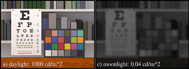
Figure 9. Time Variant Tone Mapping, eyes adjusting to light going from a light to dark area[Ferwerda96].

4. Mapping Spectra to Color and Vice Versa

Mapping Spectra to Color involves mapping Spectral Power Distribution of a light source to 3D color values like RGB, CIE XYZ, etc. The technique for accomplishing this task entails converting a continuous function that the light is represented by to one or more discreet color values. A plethora of representations for this conversion exist including direct sampling, and Polynomial representation of the light function.

Direct sampling of the function that represents the light is by far the most convenient way to convert Spectral Curves to color. To sample the Spectral Curve, the range is usually limited to approximately 380-800nm because this is the range of the Human Visual System. Then readings are taken at specified intervals of wavelength, for instance every 10nm. In most cases, this technique works well but at very small intervals in wavelength there is a huge spike in the curve. This may result in misses of important features of the light because sampling is done at sparse values.

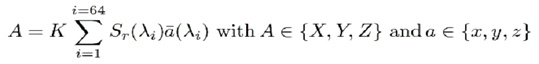
Figure 10. Sample the visible spectrum every 5nm [380-700nm], apply Riemann type integration[Rougeron97].

The Polynomial technique uses a cubic piecewise polynomial to represent the Spectral Curve of the light. This technique possesses several attractive attributes such as being able to use polynomial reduction techniques when evaluating the polynomial or any multiplication with other polynomials (light reflection). Also this technique offers flexibility when orienting the points of the polynomial to account for spike or other abnormalities of the Spectral curve of the light.

Mapping Color To Spectra involves the reverse of mapping Spectra to color. In this case, each pure color has its own Spectral Curve, so all that is required is to determine how much each color contributes to the pixel. An example of this is having three spotlights shining at the same point and each spotlight possessed an intensity knob that could be raised and lowered in intensity. All that would be required is an adjustment of the knobs until for the desired match in color was obtained. The rationale for converting back to a Spectral Curve when the RGB values are know is that certain natural phenomena can only be rendered using Spectral Rendering algorithms. These phenomenon include: Light interference (Soap Bubbles, hummingbird wings, film coated objects).

5. Spectral BRDFs

As mentioned in section 4,the need for Spectral Rendering (Spectral BRDFs) arises in a number of natural phenomena including polarization, interference, dispersion, and fluorescence.

For most purposes, it is sufficient to describe light as an electromagnetic wave of a certain frequency that travels linearly through space as a discrete ray (or a set of such rays). However, closer experimental examination reveals that such a wavetrain also oscillates in a plane perpendicular to its propagation. The exact description of this phenomenon requires more than just the notion of radiant intensity, which the conventional representation of light provides. Examples of this would be polarized filters, light reflection off of water in a body of water.

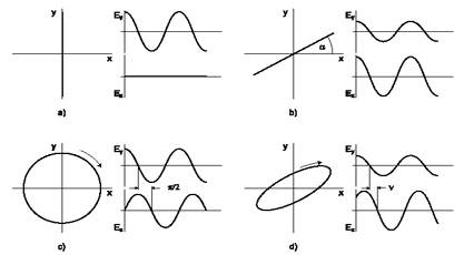
Figure 11. Four examples of the patterns traced out by the tip of the electric field vector in the X/Y plane[devlin02].

Most light interference effects observed in nature result from thin films or layers of thickness below 1mm. Light interference can occur on both the reflection side and the transmission side. This situation arises because the interfering lights have different optical path lengths.

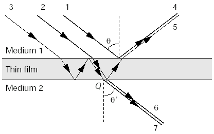
Figure 12. Light interference can occur on both the reflection side and the transmission side[sun99].

Dispersion can be seen when light hits a glass prism and is split into its spectral components, resulting in a rainbow-like effect. This effect is due to the types of materials used to split the light into its color components; these materials are referred to as dielectric materials. This phenomenon is also seen in oil slicks on top of water and in rainbows generated from light penetrating rain or mist falling in the sky.

Figure 13. Split of an incident white light beam into its spectral components in a prism[devlin02].

Fluorescence is caused by processes within the molecules that are responsible for the color of an object. The key point is that reemission of photons that interact with matter does not necessarily occur at the same energy level - which corresponds to a certain frequency and ultimately color - at which they entered.

6. Conclusions and Future Direction

Spectral Rendering is gaining momentum in the graphics industry, especially as people strive to create images that display real world phenomena as accurately as possible. Even though the hardware capabilities are not capable of rendering High Dynamic Range values (nor should they), we have algorithms and techniques for mimicking these contrasts.

So in the future of photo-realistic rendering I would expect to see all the techniques reviewed in this paper used in a wide variety of ways, all with the aim to render images as physically accurate as possible.

References:

- Devlin, Kate, State of The Art Report Tone Reproduction and Physically Based Spectral Rendering, Eurographics, 2002
- Rougeron G., P'eroche B.,An adaptive representation of spectral data for reflectance computations,Rendering Techniques '97 Proceedings of the 8th Eurographics Workshop on Rendering
- Sun Y,F. David Fracchia, Thomas W. Calvert, and Mark S. Drew "Deriving Spectra from Colors and Rendering Light Interference", IEEE Computer Graphics and Applications, 1999,
- McNamara, Ann, Visual Perception in Realistic Image Synthesis: State of the Art Report", PowerPoint Presentation/EUROGRAPHICS, 2001
- Hill, F.S., "Computer Graphics Using OpenGL", Prentice Hall, 2001
- G. Wyszecki, W. S. Stiles, "Color Science, Concept and Methods, Quantitive Data and Formulae", 2nd ed., John Wiley and Sons, (1982)